Home Depot Product Search

One of the most improtant features of e-commerce platforms is product search, which displays a list of products in a response to a user search query. The products are typically represented as a collection of properties (e.g. brand, type, size, color, etc.). A typical approach to e-commerce search is to use an out-of-the-box search engine (e.g. Apache Solr or Elastic Search) to retrieve a set of candidate products by matching user queries against properties text, and then apply a post-processing model to rerank the products. The Home Depot Product Search Relevance Kaggle competition challenged participants to build such a model to predict the relevance of products returned in a response to a user query.

Data

For the challenge Home Depot provided a dataset, that contains pairs of user search queries and products, that might be relevant to these queries. Each such pair was examined by at least three human raters, who assigned integer scores from 1 (not relevant) to 3 (highly relevant). The scores from different raters were averaged. Organizers made available instructions for human raters who judged the relevance of products to the queries, so participants can learn about the exact process used to obtain the ground truth labels.

While the user queries are simply strings, that contain one or more terms, products are more complex. Each product has a product id, title (e.g. “Delta Vero 1-Handle Shower Only Faucet Trim Kit in Chrome (Valve Not Included)”), a more verbose description (e.g. “Update your bathroom with the Delta Vero Single-Handle Shower Faucet Trim Kit in Chrome …”) and one or more attributes, which could be brand name, weight, color, etc. While some attributes have a clear name (e.g. “MFG Brand Name”), others are simply bullet points, that you might expect to see under the product description on a website (e.g. “Bullet01” -> “Versatile connector for various 90° connections and home repair projects”).

Evaluation

The goal of the challenge is to build a model to predict relevance scores for (product, search query) pairs from the test set. The quality of the model was evaluated using root mean squared error (RMSE): $\textrm{RMSE} = \sqrt{\frac{1}{N} \sum_{i=1}^{N} (rel_i - \hat{rel}_i)^2}$ , where $rel_i$ is the average human relevance score, and $\hat{rel}_i$ is the model prediction.

Data Exploration

Before making any predictions it’s helpful to look at the data to get some insights and ideas. Many participants posted their explaratory scripts and notebooks, e.g. HomeDepot First Data Exploration.

Let’s look into the distribution of relevance labels across the training set:

import matplotlib.pyplot as plt
import numpy as np
import pandas as pd
import seaborn as sns

train_df = pd.read_csv("train.csv", encoding="ISO-8859-1")
test_df = pd.read_csv("test.csv", encoding="ISO-8859-1")
sns.countplot(x="relevance", data=train_df, palette="Greens_d")
plt.show()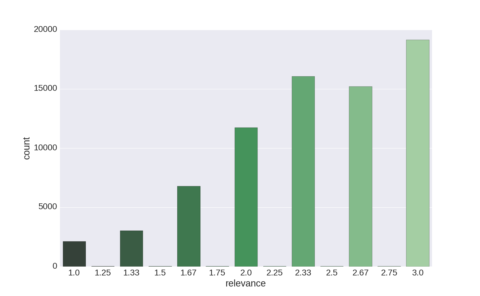

Histogram of relevance scores

As we can see, most of the products in the dataset are relevant to the corresponding queries, and the average relevance score is 2.38 (median = 2.33).

Next, let’s see what percentage of products occur in train, test or both datasets:

# Using matplotlib_venn library: https://github.com/konstantint/matplotlib-venn
from matplotlib_venn import venn2
venn2([set(train_df["product_uid"]), set(test_df["product_uid"])],
	set_labels=('train', 'test'))
plt.show()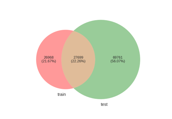

Venn diagram of products in train and test sets

And the same for queries:

# Using matplotlib_venn library: https://github.com/konstantint/matplotlib-venn
from matplotlib_venn import venn2
venn2([set(train_df["search_term"]), set(test_df["search_term"])],
	set_labels=('train', 'test'))
plt.show()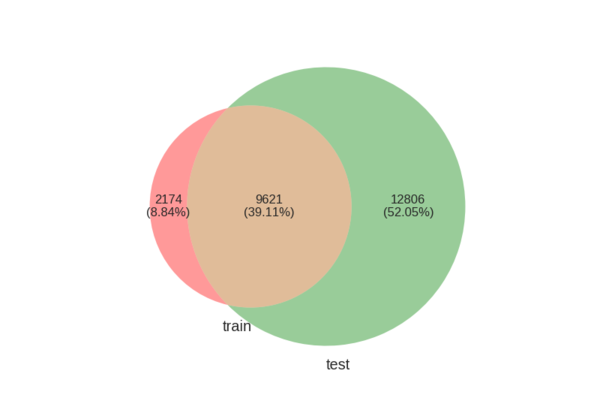

Venn diagram of queries in train and test sets

These percentages are actually quite important. It’s natural to expect that predictions for new products and queries might be harder to make, than for queries and products which the model has seen during training. Therefore, a good training-validation splits (or cross-validation splits) would maintain the ratio of repeated and new queries and products. Otherwise, the parameters tuned on the validation set can be far from optimal, and we will get a lower leaderboard score.

An interesting observation was made by some of the participants, who looked at the relevance scores for products with different product ids:

# Split products into buckets based on their product_uid
train_df["bucket"] = np.floor(train_df["product_uid"] / 1000)
sns.pointplot(x="bucket", y="relevance", data=train_df[["bucket", "relevance"]])
plt.show()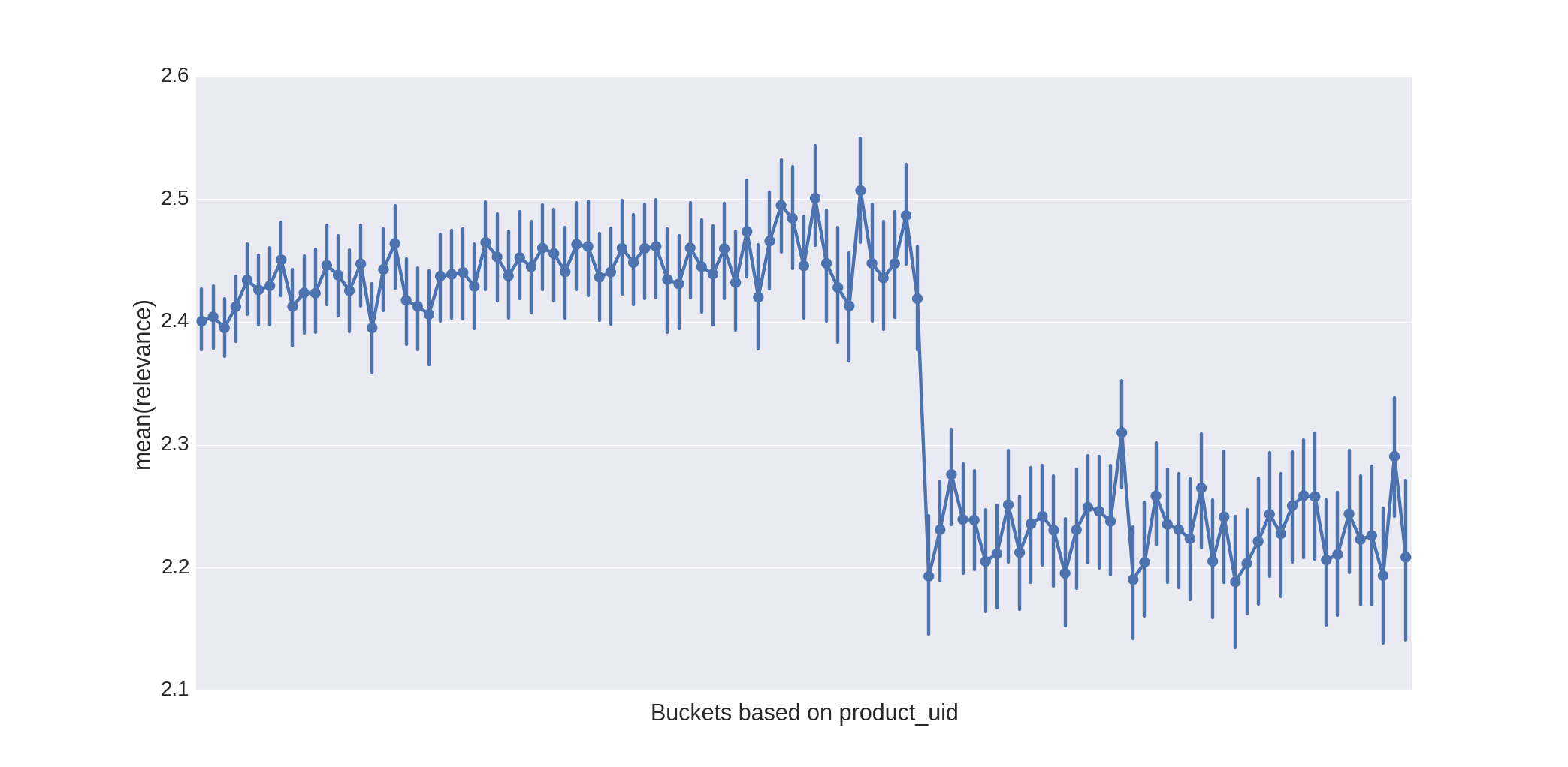

Histogram of relevance scores for different product_uid

This unusual dependence between relevance and product ids was also exploited, e.g. by adding the id itself or a binary indicators as features.

Pre-processing

A quick look at raw queries and product descriptions reveals several typical problems, that might affect the performance of a model:

Quite often queries contain typos, which can cause problems, for example, for counting the number of query terms matched in the question. Example queries: “lawn sprkinler”, “portable air condtioners”, etc. There are some typical typos, that occur again and again in the dataset, and one simple approach was to build a list of terms that frequently occur in queries, but doesn’t occur in product descriptions and manually fix these names. It’s also not hard at all to implement your own spelling corrector, e.g. spelling corrector described by Peter Norvig. Another approach was to collect spelling corrections using Google.
Products have many numeric characteristics with different units. Unfortunately, the ways these numbers and units are written in products and queries isn’t standardized. Most of the participants normalized these measures and units manually, for example:

def fix_units(s, replacements = {"'|in|inches|inch": "in",
                    "''|ft|foot|feet": "ft",
                    "pound|pounds|lb|lbs": "lb",
                    "volt|volts|v": "v",
                    "watt|watts|w": "w",
                    "ounce|ounces|oz": "oz",
                    "gal|gallon": "gal",
                    "m|meter|meters": "m",
                    "cm|centimeter|centimeters": "cm",
                    "mm|milimeter|milimeters": "mm",
                    "yd|yard|yards": "yd",
                    }):

    # Add spaces after measures
    regexp_template = r"([/\.0-9]+)[-\s]*({0})([,\.\s]|$)"
    regexp_subst_template = "\g<1> {0} "

    s = re.sub(r"([^\s-])x([0-9]+)", "\g<1> x \g<2>", s).strip()

    # Standartize unit names
    for pattern, repl in replacements.iteritems():
        s = re.sub(regexp_template.format(pattern), regexp_subst_template.format(repl), s)

    s = re.sub(r"\s\s+", " ", s).strip()
    return s

As we all know, words have different forms: singular and plural, verb forms and tenses, etc. All these variations can cause us troubles with word comparisons. A common strategy to deal with these situations is to stem words, i.e. reduce word forms to their roots. We can replace the original product descriptions and queries with stemmed versions, which should make any word comparisons more robust. There are multiple algorithms to do it, implemented in different languages. In Python one can use the nltk library:

from nltk.stem.porter import *
from nltk.tokenize import word_tokenize

stemmer = PorterStemmer()
text = [stemmer.stem(word.lower()) for word in word_tokenize(text)]

Features

Now, as we pre-processed the data, we can switch to feature engineering. The task is to estimate the relevance of the product to the given query, or in other words if the given product is a good match for the query.

The first idea is to count how many terms of the query match in the product description. One way to do this is to represent a product and query as bag-of-word vectors, where each dimension corresponds to a particular term in the vocabulary. Then we can compute cosine similarity of these vectors. However, as you can imagine the word “the” is less interesting than the word “conditioner”. A common way to estimate word importance is to compute its inverse document frequency. IDF scores could be incorporated into product or query word vectors (see tf-idf). Information retrieval research knows many other retrieval metrics besides tf-idf, for example: BM-25, divergence from randomness, sequential dependency model, etc. I’m not aware if any of the participants experimented with these models.

Unfortunately, these IR measures by default consider synonyms as different words and don’t account for word relatedness. There are different strategies, that allow one to account for semantic similarity of words: WordNet synonyms, hypernyms and hyponyms can be used to check if a word is related to another one, or we can use some kind of distributed word representation. Distributed word representations map terms to vectors in lower dimensional space (compared to the size of the vocabulary). In this lower dimensional space the distance between vectors, corresponding to related terms, is lower than for some unrelated terms. To build such representations one can use certain dimenstionality reduction techniques such as Latent Semantic Analysis, or neural network based word embeddings, e.g. Word2Vec or GloVe. The later already contain pre-trained word vectors, which you can simply download and start using. For Python enthusiast we can recommend to take a look at the gensim library, which has LSA, word2vec and other similar models implemented.

A particularly neat idea to compute similarity between longer pieces of text given word embeddings is so called word movers distance. The idea of this method is borrowed from the earth movers distance and it estimates the total “effort” required to move words of one piece of text, e.g. query, to the other, e.g. product description. The wmdistance method in word2vec class from gensim implements this algorithm. Here is a short example:

from gensim.models import Word2Vec
from nltk.corpus import stopwords

# Load word2vec model
model = Word2Vec.load_word2vec_format('GoogleNews-vectors-negative300.bin.gz', binary=True)
# Normalize the embedding vectors
model.init_sims(replace=True)

# Prepare sentences
stop_words = stopwords.words('english')
sentence1 = [w for w in "portable airconditioner".split() if w not in stop_words]
sentence2 = [w for w in "spt 8,000 btu portable air conditioner".split() if w not in stop_words]

print 'Word movers distance = %.3f' % model.wmdistance(sentence1, sentence2)

As we noted earlier, user queries contain a lot of typos. One idea was to fix the typos as the pre-processing step. Alternatively (or in addition), we can use fuzzy string matching. We can allow terms to match if their edit distance is less than a certain threshold, or we can count character n-gram instead of complete term matches. More specifically, instead of splitting query and product description into words, we can split into character n-grams (e.g. 3,4,5,6-grams). This bag of n-grams can be used similarly to bag of words, e.g. to compute cosine similarity or simply the number of matched n-grams.

Another useful idea is that not all parts of the product description and of the query are equally useful. It was noted, that matched types of products and brands are very useful for predicting the product relevance. A good strategy is to have different features for matching some specific attributes, e.g. product type, brand, size, color, etc. The model can then learn different weights for different types of matches. Unfortunately, these attributes are not always implicitly given. The product attributes file contains a mixture of various textual information. Therefore, some heuristic rules can be used to extract color, size (e.g. dictionary of colors, presence of some specific units), etc. The brand attribute was actually given:

attributes_data = pd.read_csv(attributes_path, encoding="ISO-8859-1").dropna()
brand_data = attributes_data[attributes_data['name'] == 'MFG Brand Name'][["product_uid", "value"]].rename(
	columns={"value": "brand"})

Besides that one can imagine that matched adjective, such as “portable”, might be less important than a matched noun, e.g. “conditioner”. Therefore, we can use a tagger to annotate words in product descriptions and queries with their part-of-speech (POS) tags. Luckily, Nltk library, which we used before for stemming, has a POS tagger (here is the list of part-of-speech tags):

import nltk
text = nltk.word_tokenize("And now for something completely different")
nltk.pos_tag(text)
# Returns
# [('And', 'CC'), ('now', 'RB'), ('for', 'IN'), ('something', 'NN'), ('completely', 'RB'), ('different', 'JJ')]

Finally, let me describe some insight from the interview of the winners of this challenge. As we have seen in the exploratory analysis, many of the queries appear multiple times, so do products. So, for a random test instance there is a chance that we had some instances with the same query or product in the training data. We would like to use this somehow. The winning team clustered the products for each query and computed cluster centroids. Then, at test time they computed the similarity of the current product to the query centroid and used this as a feature. Please refer to the winning team interview for details.

Of course, this is just a small set of features that can be and were used to represent product-query pairs for relevance prediction. Many of the participants shared their detailed list of features on the HomeDepot competition forum.

Algorithms

Most of the participants of the challenge posed this problem as a regression problem, i.e. predicting a numeric relevance score. Participants explored many different algorithms: from linear regression to random forest and gradient boosted regression trees. Top scoring teams didn’t stop here, and as common in Kaggle competitions, built an ensemble of different approaches. The winners of the competitions stacked three layers of models. On the lowest layer they build 300 different regression models using various combinations of features. On the next layer 63 models combined predictions of the lowest layer models, and finally these 63 models were combined into a single model using ridge regression. Here is an overview of the winner model architecture, taken from the Kaggle interview post 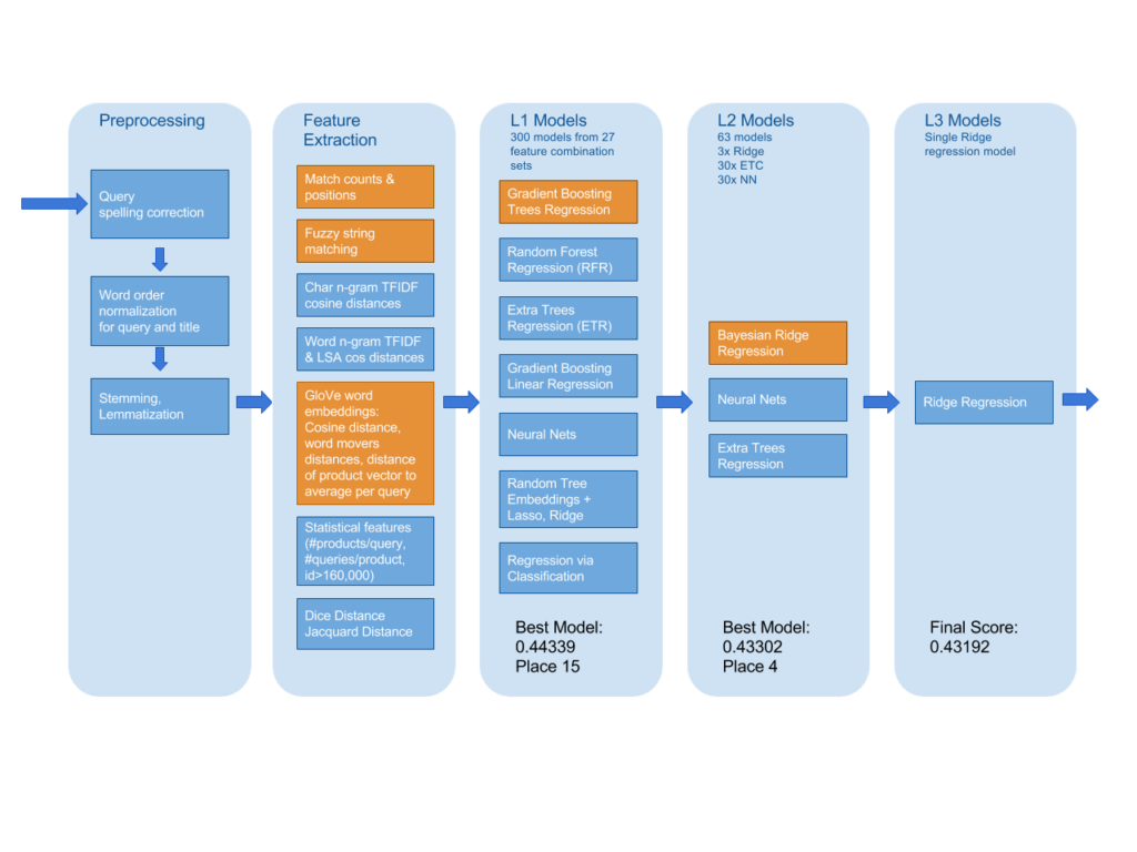Overview of the winning approach from Home Depot Kaggle challenge. The image is taken from http://blog.kaggle.com/2016/05/18/home-depot-product-search-relevance-winners-interview-1st-place-alex-andreas-nurlan/

Conclusion

To conclude, Home Depot Kaggle challenge provided a nice and very practical problem from the area of e-commerce. We hope the ideas, described in this post and provided links, were helpful and gave you a glipse into ideas that work well in practice for product search kind of problems.

“To alcohol data! The cause of, and solution to, all of life’s problems.” © Homer J. Simpson